OHDSI Home | Forums | Wiki | Github

Building a validated OHDSI outcome library

Hi all. I wanted to help structure the discussion on this topic a bit, and add my 2 cents:

Note: I’m here deliberately avoiding the term “phenotype”, because recently people have stressed that a phenotype is a set of people with certain characteristics. An outcome on the other hand is an event that occurs in peoples’ lives, and most importantly has a date of onset, whereas a phenotype does not.

Because the data we have often was not collected for the purpose of research, many things we need to know for our analyses are actually not explicitly recorded. This is most pressing when it comes to what we call ‘outcomes’: events that happen in patients’ lives that are either good or bad, may have been caused by something else, and perhaps could have been predicted and/or prevented. To construct outcomes for our analyses, we therefore often rely on complicated logic that uses the data we do have. For example, if we want to find people who have experienced an acute myocardial infarction, we may require diagnosis codes in combination with procedure codes for the diagnostic tests, and maybe even treatment codes. The question remains: what is the right set of logic, and how well does a specific set of logic perform in terms of sensitivity and specificity?

In the past, work in OHDSI has focused on learning the logic from the data, but that had some mayor limitations, such as strong requirements on the data, and not being able to pinpoint the date of onset of the outcome.

So now we’re considering using manually crafted cohort definitions based on expert knowledge, as is the status quo in observational research, and finding better ways of evaluating these. I’ve created a Venn diagram in Figure 1, showing the group of people that truly have the outcome, and the group of people in a cohort (e.g. meeting an ATLAS cohort definition). Based on the insersection (true positives) of the two groups, and the number of people in one group but not the other (false negatives and false positives), we can compute important performance metrics such as sensitivity and specificity.
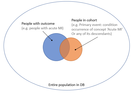
Figure 1. People with the outcome and people in the outcome cohort.

One way to estimate these numbers is to perform chart review: we go back to the original data, read the doctor’s notes, and investigate further to determine with high certainty whether someone really had the outcome. Because this is a lot of work, we typically take a random sample. We could take a sample of the entire population in the database, as this would allow us to compute both sensitivity and specificity. But the outcome is usually rare, and we would therefore need to review a large sample to have some people with the outcome, wasting valuable resources reviewing charts of people who certainly do not have the outcome, as depicted in Figure 2.
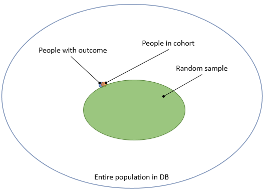
Figure 2. Taking a random sample from the entire population.

To avoid this problem, the typical approach is to take a sample of people that are in our cohort, as depicted in Figure 3.
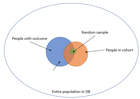
Figure 3. Taking a random sample from the people in the cohort.

The downside of this is that it only allows computation of the positive predictive value (PPV), which is not really what we want to know.

@nigam wrote this proposal to allow computing sensitivity and specificity using a small sample. The basic idea is depicted in Figure 4. (@nigam: please correct me if I’m wrong) Select a group of people that definitely have the outcome (e.g. people that get the treatment for the outcome), and call this set E. Sample 100 people from this group. In addition, sample 100 people that are neither in E nor in the cohort. People in the first 100 are likely to have the outcome, and many will be in the cohort. People in the second 100 are likely not to have the outcome, and are by definition not in the cohort, so all 4 cells of the 2-by-2 table we need will have some data.
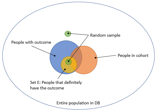
Figure 4. Computing sensitivity and specificity using two small targeted samples.

@jswerdel proposed a different approach: identify a group of people that certainly have the outcome (e.g. people with 5 diagnosis codes), and call this the xSpec (extreme specificity) cohort. Typically, this is a subset of the cohort we’re trying to evaluate. Then, fit a model that predicts whether someone is in xSpec or in the general population. The nice thing about this is that it creates a gradient membership: a lot of people have a predicted probability > 0, but only a few will have a high probability. Joel then proposes identifying the ‘inflection point’ where this probability changes rapidly, and declare everyone with a higher probability than this point to truly have the outcome. This allows us to compute the sensitivity and specificity without performing chart review, and is depicted in Figure 5.
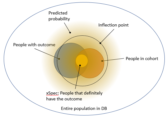
Figure 5. Using a predictive model to separate true from false.

I like Joel’s approach in that it is automatic, and gives an approximate answer without requiring extensive chart review.

My two cents:

My concern with Nigam’s proposal is that it focuses entirely on the extremes, but not on the middle-ground. Probably everyone in the first 100 have the outcome, probably everyone in the second 100 do not have the outcome, so most of the effort is wasted in confirming the obvious.

My first concern with Joel’s proposal, which becomes apparent in Figure 5, is that xSpec might not be at the ‘center’ of the true population with the outcome, and drawing a larger ‘circle’ around it may not fully coincide with the true population. To move from the abstract to a concrete example: imagine xSpec by its definition only includes people that have an MI and then are rushed to the hospital. It may then miss the characteristics of people that have an MI while already in the hospital (just making this up). Another concern is that the inflection point seems pretty arbitrary, although Joel has done some empirical validation there.

One idea that combines Joel’s and Nigam’s: If we want to do chart review, why not focus on the group of people with the highest ‘information’ (in information theory sense)? Sample from the entire population, but give higher sample probability to those people that Joel’s model indicates are ‘on the fence’, so neither certainly without the outcome, or certainly with the outcome. We can later even correct for this weighting to apprimate an unbiased sample.

Anyway, just hoping to keep the discussion moving forward. I think building a validated outcome library has the highest priority, and appreciate everyone working on this!

1 Like

Interesting and very important topic, indeed.
I have an experience linking national claim data with hospital EHR data. I think we can also validate the performance of algorithm by linked data
(The linked data contains records from sampled patients who had a history of percutaneous coronary i ntervention)

The other cohort I want to identify is the ‘cause of death’
Korean claim data has the data for the cause of death, and I converted those data into CDM (so we have labeled data).
Can we develop an algorithm to identify cardiovascular death from all mortality?

Great summary and diagrams, @schuemie.

I had proposed stratified sampling, based on the observation that if you have a second technique that classifies well (even if not independent) then your sampling becomes more efficient. A few comments first.

In genetics, phenotyping usually refers to a permanent characteristic. In informatics, it can be timed. So we can call it whatever we decide, but having a date of onset is consistent with an informatics phenotype. I see outcome as more specific than phenotype not because of the use of a time, but because it implies that it was caused by something else we are interested in, as opposed to a disease that just happens.

Even having a pathognomonic treatment does not guarantee the disease until you have measured the rate at which the treatment is falsely stated in the record. The bigger question is about the five codes. Harvard measured the PPV for having five ICD codes and it was about 0.85 not 1 (I forget the disease now, might have been rheumatoid arthritis). Therefore, with any method, we can either confirm the accuracy with sampling and review, or simply state a reasonable range based on experience. For Joel’s five-code method, you are just building a model, so PPV 0.85 might be enough to build a model that is then used to stratify for further sampling.

I think @nigam was trying to solve what we can do with no chart review. So the treatment gives us an estimate of sensitivity, but it may be biased because only more severe cases may get treatment. But it is still good for a free ride. (Or nearly so if you just do a small review for PPV to complete the picture.)

Your Figure 4 is stratified sampling. I just used simulation to show that you can achieve the same CI on sensitivity, specificity, and PPV with fewer reviewed cases if you stratify by a second predictive method, even if that method is not independent. The problem with Figure 4 is that the green circle in the white area is no better than Figure 2 in terms of estimating sensitivity that is missed by the treatment. I.e., if there is no treatment bias, then you don’t need that green circle, and if there is treatment bias then it is a lot of work to measure the sensitivity.

I saw @jswerdel’s approach as providing a continuous range from which to stratify (with the option to go dichotomous at the inflection point), which is what you point out at the bottom.

In practice, I find that reviewing ten cases selected by the outcome algorithm goes a long way in telling you how this is going to go. Are there a lot of mistakes, are these all very severe cases, etc.

Once we do this for some number of outcomes, then I suspect we would be able to assert a reasonable range of performance with much less review or no review. E.g., we would know, on average, how often pathognomonic treatment went off base.

George

Great summary. I can’t see the utility of the method described in figure 4. I think the yellow circle is enough to estimate the sensitivity and specificity if the so-called “definitely” outcome is a parallel phenotyping strategy independent from the phenotyping algorithm to define the patient cohort. If this is not a parallel phenotyping algorithm, then we may not use the 2-by-2 table to calculate the sensitivity and specificity. IMHO

Nice summary @schuemie! Yes, a “hard” boundary for set E, and random
sampling as shown in figure 4 is suboptimal, and combining with the xSpec
idea to have informed / stratified sampling (i.e. sample based on
information we might get from reviewing the record) definitely makes sense.
George also proposed that (without the pictures though!).

Bottom line: we need a clear way to define set E (ideally as a continuous
range; and we can then stratify or go dichotomous).

The challenge is we might not have good ways to define that set (i.e. xSpec
is not perfect, using treatment as as surrogate is not perfect). All these
approaches hinge on being able to stratify by a second method (and the
quality of that second method). This is where George’s suggestion of
sampling a few cases flagged by this other method can inform us on whether
our automated estimation of sensitivity, ppv, specificity etc is going to
work or not.

ps: superb figures! I was going to try and make visuals, but now will reuse
these :-).

Nigam.

dear martijn,

when you say that PPV ‘is not really what we want’, you are in fact rejecting a very useful input. indeed, PPV and all the other indices are analytically linked, so that information on any of them can be used to derive the others. have a look at the second column of this poster from last autumn’s symposium.

the proposal that you make here combines with the ‘components’ strategy, that i have been working on in several european projects. the core idea is trying and split the cohort in subcohorts which can be assumed to be internally homogeneous wrt validity. have a look at this second poster with 3 examples (AMI, T2DM, pertussis) from a bunch of databases. subcohorts are systematically characterised by 3-4 dimensions, which are associated to validity.

cheers, rosa

Thank you @schuemie, this is an excellent post to get our community to
rally around formalizing our objective for cohort definition and
evaluation. I hope others can contribute here so we can develop a explicit
plan of attack to research and develop strategies that can ultimately
become a new community best practice.

Just to add a little bit to the scaffolding before jumping too far into
@nigam and @jswerdel nice candidate approaches:

In OHDSI, we have defined a cohort to be a set of persons who satisfy one
of more inclusion criteria for a duration of time.

This cohort definition has several important implications.

  1. A cohort is based on timestamped clinical observations in a database.
    These clinical observations are merely proxies for the true heath state of
    a patient at any moment in time, and some of those proxies are more or less
    reliable than others. Ex: A pharmacy dispensing record is a proxy in
    claims data for a patient’s drug exposure, but we don’t actually have true
    evidence of when or how much the patient actually consumed, or how the drug
    was metabolized in the body. It is often tempting to get lazy in
    describing a cohort by the phenomenon we seek to find vs, the proxies we
    use to infer the phenomenon (ex: ‘persons with diabetes’ vs. ‘persons with
    a health encounter where a diagnosis code of diabetes was recorded’), but
    its exactly this distinction that results in cohort misclassification
    error. There may be people who have the phenomenon of interest who don’t
    have the proxies (false negatives) and people who don’t have the phenomenon
    of interest but do have the proxies (false positives).

  2. A cohort definition is temporal in nature. So, it would be incomplete
    to say a cohort is ‘persons with diabetes’, because that description does
    not convey the notion of when the persons enter and exit the cohort. A
    more complete definition could be: ‘persons with diabetes, who enter at
    the time of their first diagnosis of the disease and exit at the end of
    their observation period’, or ‘persons who have continuous enrollment from
    Jan2017 to Dec2017, who have a diagnosis of diabetes during that time’.
    Note, just because the cohort is temporal, doesn’t mean the use of the
    cohort requires the temporality. Some expected cases: 1) often when we
    define an ‘outcome cohort’, we care about cohort entry, but are less
    concerned with cohort exit (for example, when we’re doing a
    population-level effect estimation study that examines a time-to-event
    relationship). 2) if you were doing genome association studies, we
    (currently) believe your genetics are constant and determined at birth, so
    relating a SNP to a disease has an implicit temporal relationship (e.g.
    gene preceded disease) that is not required to be explicitly modeled.
    However, when we are in a situation where the temporality information
    (either cohort entry or cohort exit) is analytically important, there is
    another potential source of error: misspecification of the cohort
    entry/exit date.

For purposes of this rant, I’m going to table the date misspecification
problem to focus on the misclassification error, but I don’t want us to
lose sight of that other source of error indefinitely:

The extent of misclassification error of any given cohort can be fully
characterized by 3 metrics: sensitivity (the proportion of true cases
correctly identified as a candidate case by a cohort definition),
specificity (the number of false cases correctly identified as not a
candidate case by a cohort definition), and positive predictive value (the
proportion of cases identified as a candidate case by a cohort definition
which are correctly true cases). With these 3 metrics in place, the entire
confusion matrix can be computed to quantify the number of ‘true
positives’, ‘false positives’, ‘false negatives’ and ‘true negatives’ in a
given population, and also to yield other associated metrics, such as:
prevalence, accuracy, and negative predictive value. Each of these three
metrics provide complementary information about the extent of
misclassification, but each on their own is insufficient. @rosa.gini had a
nice poster that showed the relationship between the various metrics at
last year’s OHDSI Symposium.

@jswerdel did a nice job of presenting on the OHDSI community call a few
weeks back about the current challenges in ‘validation’ that is seen in the
broader research community to date (
https://drive.google.com/file/d/1VuzO4nPlxHiOSBa-4LVOcdk8_CKMQlV0/view?usp=sharing).
He highlighted the work of Rubbo et al. (
https://www.ncbi.nlm.nih.gov/pubmed/25966015), who performed a systematic
review of validation efforts of the outcome of myocardial infarction;
amongst the 33 ‘validation’ studies identified, all reported positive
predictive value, but only 11 reported sensitivity and 5 reported
specificity. I think these results are generally representative of
validation work at large, where the prevailing approach to ‘validation’ for
most cohort definitions focuses on some sampling of candidate cases with
clinical adjudication through source record verification, which can provide
an estimate of positive predictive value. But positive predictive value
alone, without accompanying estimates of sensitivity and specificity, is
not directly actionable, because it doesn’t speak to how many cases are
‘missed’ (e.g. false negatives). Bush et al. (
https://www.ncbi.nlm.nih.gov/pubmed/29405474) recently showed how
alternative cohort definitions can reflect tradeoffs between PPV and
sensitivity, further underscoring the need to estimate both.

As an analogy, we see in the machine learning community, as is currently
applied as part of the best practices out of our patient-level prediction
workgroup, one commonly used measure of discriminative accuracy is Area
Under Receiver Operating Characteristic (AUROC) curve, which can be
described as the integration across the potential tradeoffs between
sensitivity and specificity at all possible threshold values. Depending on
your perspective, AUROC has the advantage or disadvantage of being agnostic
to the prevalence of the target condition. Another metric for evaluating
discrimination in prediction work is Area Under Precision-Recall Curve
(AUPRC), which can be described as the integration across the potential
tradeoffs between sensitivity (recall) and positive predictive value
(precision) at all possible threshold values. Depending on your
perspective, the AUPRC has the advantage or disadvantage of being
conditionally defined by the prevalence of the target condition. In
prediction, neither AUROC or AUPRC are ‘right’ or ‘wrong’, but rather they
provide complementary information, because together they represent all 3
necessary metrics: sensitivity, specificity, and positive predictive value.

So, the first assertion I would like to make is that we need a cohort
evaluation process that can provide estimates of sensitivity, specificity,
and positive predictive value. So, source record verification of a sample
of candidate cases would not be a sufficient process on its own, because it
only provides PPV. But it does represent one possible approach to produce
one of the estimates we need. There may be other approaches that can also
estimate positive predictive value, and it is worthwhile for us to develop
and evaluate those alternative approaches because we know source record
verification is very resource-intensive, not fully reproducible, and
increasingly problematic as the EHR data becomes the only ‘source’ to
verify against. @jon_duke and his team shared their work at last year’s
symposium in allowing electronic record verification via patient profile
annotations, and that seems like a promising direction for reducing the
resource burden of clinical adjudication, so I’m eager to see that work
completed and rolled into the OHDSI ecosystem. @jswerdel’s approach
represents an orthogonal approach to empirically estimate positive
predictive value without clinical adjudication.

But beyond building a better mouse trap for the part of the problem for
which we have an approach (PPV estimation), we need to also devote time and
attention to researching and developing methods that estimate sensitivity
and specificity. This is why I’m so excited by the work that @nigam and
@jswerdel are proposing, because it’s almost always infeasible to do source
record verification on a sufficient population sample to yield reliable
sensitivity/specificity estimates. @schuemie provides some valid concerns
about both approaches, which I share, but I think its important to frame
the context here: the first-order problem we need to solve is a shared
recognition that sensitivity/specificity/PPV need to be estimated in order
to quantify the misclassification error. The second-order problem we’re
now talking about is whether there may be systematic error in the method
that we use to estimate the sensitivity/specificity/PPV, meaning we have a
estimate but we don’t know if its biased and may need a broader perspective
to reflect our inherent uncertainty that goes beyond the sampling
variability in most current confidence interval calculations.

To that end, one reflection that may or may not be useful: we have three
different metrics that we are trying to estimate: sensitivity, specificity,
and positive predictive value. Clearly, the ‘true’ value of these metrics
are highly dependent on one another, but I’m not convinced that this means
that whatever approaches we develop to estimate each of the three metrics
has to account for this dependence. Instead, we could frame three
independent research opportunities:

  1. Develop a process to estimate the proportion of true cases that a given
    cohort definition identifies (sensitivity), and evaluate its operating
    characteristics (e.g. accuracy and precision of the sensitivity estimate)
    and efficiency (e.g. resource requirements, assumptions/constraints).

  2. Develop a process to estimate the proportion of false cases that a given
    cohort definition correctly fails to identify (specificity), and evaluate
    its operating characteristics (e.g. accuracy and precision of the
    specificity estimate) and efficiency (e.g. resource requirements,
    assumptions/constraints).

  3. Develop a process to estimate the proportion of cases identified as a
    candidate case by a cohort definition which are correctly true cases
    (positive predictive value), and evaluate its operating characteristics
    (e.g. accuracy and precision of the PPV estimate) and efficiency (e.g.
    resource requirements, assumptions/constraints).

It could very well be that our ‘best practice’ might ultimately involve one
or more different processes for each metric. I think it will be a
tremendous contribution to the field at large when we build a cohort
definition library, where each human-readable and computer-executable
definition is accompanied by the characterization statistics and cohort
evaluation metrics against the OHDSI network of databases. But I expect
it’ll prove even more valuable when we also provide the field a clear
cookbook for how to follow ‘best practice’ to define and evaluate the next
cohort that can then be added into the library. Give a man a fish and you
feed him for a day; teach a man to fish and you feed him for a lifetime.

dear patrick,

actually the formulas in my poster are not something you need to account for: they are an opportunity for you to work less to obtain the same information :smile:
indeed, if you have PPV already, you don’t need sensitivity AND specificity. you just need one among sensitivity and specificity, and the other is analytically derived. or, if you happen to have some external information on the prevalence of your cohort on the study population (were false negatives live), you don’t need anything else.

le me show it explicitly. call P the observed prevalence (this is something you know, because it is observed), pi the ‘true’ prevalence (which may be unknown), SE the sensitivity and SP the specificity. then from the formulas you can quickly see that, if you have PPV and SE

SP=1-(PxSEx(1-PPV))/(SE-PxPPV)

on the other hand, if you have PPV and pi

SE=P x PPV/pi
SP=1-(Px(1-PPV))/(1-pi)

so: life is easier! :smile:

(this was presented at ICPE, and is currently submitted for publication, but actually it is just solving the system in the poster)

Thanks everyone for a great discussion! I agree with Patrick that the most important thing is to recognize that both sensitivity, specificity as well as PPV need to be estimated.

In the OMOP Experiment we showed that lower PPV doesn’t necessarily come at poorer performance of estimation methods. This is especially true when a small decrease in PPV comes with a huge increase in sensitivity. The current status quo of focusing solely on PPV (searching where the light is, instead of where you lost your keys) has, in my humble opinion, lead to overemphasizing this metric at the cost of the others.

I did not mean to suggest we should not go forward with @jswerdel and @nigam’s ideas. In fact, I’m eager to see their research move forward, and am happy to help where needed.

Yup, good discussion. Overall, it all boils down to two choices:

(1) What is the way we define set E (via a heuristic, which gives a hard
boundary or via a model that gives a probability of membership)
(2) How do we sample from set E, and outside of set E. (i.e. stratified
sampling across probability bands, or using a couple of heuristics to
define multiple set E (and not E) instead of just one).

If we can make these choices clear, record them, and require that people
report the choice as well as the performance metrics of a phenotype
definition we have made progress.

Thanks @rosa.gini. Yes, to clarify in case I may have caused confusion:
I am not advocating that we must independently estimate sensitivity,
specificity, and positive predictive value. Rather, we want to obtain
estimates for sensitivity, specificity, and positive predictive value, and
we should have the freedom to derive them in whatever way we determine is
most efficient and provides the most reasonable estimate. To fill the
confusion matrix for a given population, you need four pieces of
information, two of which are directly observable: 1) the number of persons
in the overall population, and 2) the number of persons who satisfy the
cohort definition. You are absolutely correct, that if you estimate
positive predictive value and sensitivity, then it is possible to derive an
estimate for specificity (and also estimate the ‘true prevalence’). So too
it is true that you could derive an estimate of positive predictive value
using sensitivity and specificity, or derive a sensitivity from PPV and
specificity. And as you point out, if you could generate a reliable
estimate of the true prevalence, that it can be possible to derive two of
the three metrics (sensitivity, specificity, PPV) given one estimate. My
point is raising this flexibility is because I don’t think we should
necessarily presume positive predictive value has to be one of the metric
estimated, not should we presume source record verification is our only
method to yield a PPV estimate. I’m quite confident that if we continue to
focus on the phenotype evaluation problem, that we can likely develop
multiple alternative creative solutions, as @nigam, @jswerdel, and
@rosa.gini’s work already suggests.

dear patrick,

i am happy we are on the same page!

let me just spend an additional word on the neglected Negative Predictive Value (NPV). this is the share of people outside of the cohort who are correctly non cases. this index has the same informative content as the other three (so, if we have NPV and one of the others, we have everything). the truth is, in many cases NPV (as well as specificity) is so close to 100%, that it is very difficult to estimate precisely enough. on the other hand, if prevalence of the condition is sufficiently high and sensitivity is not perfect, it becomes a more reasonable parameter to estimate, and there may be situations when it is more practical to estimate than other validity indices.

in summary, if the plan is to set up processes to estimate validity parameters, i would suggest to do so for the four musketeers - all for one and one for all :smile:

cheers, rosa

Good afternoon everyone,

I was introduced to this conundrum of phenotype evaluation last month at our F2F. I very much enjoyed participating there and appreciate the ongoing discussion in this forum here. I was also pleased to meet many of you at the event.

With our predilections for Venn diagrams in mind, I was curious about the extent to which @nigam’s @jswerdel’s, and @rosa.gini’s work compares/contrasts. Is the idea to work on the methods separately and have multiple tools at our disposal, or is there an interest in eventually developing a single unified solution through a collaborative working group?

Also, are there others in our community currently working on this problem?

Thanks,
Aaron

Hi all,

Just wanted to share these two papers I stumbled on to:

“Enabling phenotypic big data with PheNorm” describes a fully automated system for generating phenotype definitions. In some ways it is similar to the work by @nigam, @jswerdel and others, in that it focuses on predictability of a group of people (i.e. the cohort).

The system mentioned above makes use of the work described in “Surrogate-assisted feature extraction for high-throughput phenotyping”, which mines existing knowledge sources to identify relevant features, rather than rely on the observational data alone.

1 Like
t