Moving a discussion with @aschuler from e-mail to the forums. The main discussion is on whether positive controls should be synthesized by adding outcomes on top of negative controls (only during exposure to the drug of interest), or by simulating all outcomes.
Alejandro argued:
For one, even the “true negatives” are not perfectly “true”. If that’s the case, the “true” counterfactuals (i.e. the observed outcomes, duplicated) are not the true counterfactuals. However, the “truer” the negative, the truer the counterfactuals and the closer you get to the desired effect. If you can make a strong argument for your true negatives, or at least some of them, then this shouldn’t be a huge issue, although it’s important to acknowledge it.
The second problem is that you are using negative data (data for exposure-outcome pairs where there is no effect) as a stand-in for positive data. There is no rule that the confounding structure (observed or not) that is present in negative data is the same as that which is present in positive data, so using these signal-injected datasets to find methods that will work for positive associations is not foolproof. This is also probably not a killer downside- in aggregate I think that there are enough negative datasets that share confounding structure with positive datasets that it should all even out.
The final issue is related to the problem with my method, which is that it cannot perfectly capture the structure of the unobserved confounding. Although you are only changing some of the outcomes, doing that is still disrupting the unobserved confounding structure, just like my method is doing. The bigger the desired effect size, the more outcomes you will change and the more the unobserved confounding structure will be disrupted. My method has the exact same problem, which we discussed yesterday, but I think both methods address it: yours by leaving as many outcomes untouched as is possible, and mine by applying the minimum possible perturbation to the outcomes in aggregate such as to produce the desired effect size. It’s really the same idea: the less you move the data, the less you perturb the unobserved confounding. With binary outcomes, the two methods should largely produce the same result! And with either approach, artificially removing features to simulate unobserved confounding would do even more to convince us that the evaluations are legitimate- a critic would have to argue that there is some unobserved variable that has a confounding relationship that is totally different than the confounding relationships present in any of the observed variables in order to invalidate this approach (and that’s assuming the total annihilation of the unobserved confounding structure, which we know neither method does).
The first two (ideally minor) issues do not apply to my method, and I think I’ve adequately laid out the case that both methods are equally susceptible to the third issue, and that both do their best to address it. That leaves my method at 2.75/3 issues addressed, and the signal injection at 0.75/3?
And later:
Ah, and I also just realized that even if the true negative datasets really do have 0 average treatment effect, that doesn’t mean there isn’t heterogeneity present! If there is heterogeneity (even minor), then again you do not really know the patient-level counterfactuals and thus the signal injection will not give you the treatment effect you think you’re getting.
Thanks @aschuler! These are all good points. Let me at least try to respond to your first one: are negative controls truly exactly null? I’ve tried to answer this question with some data.
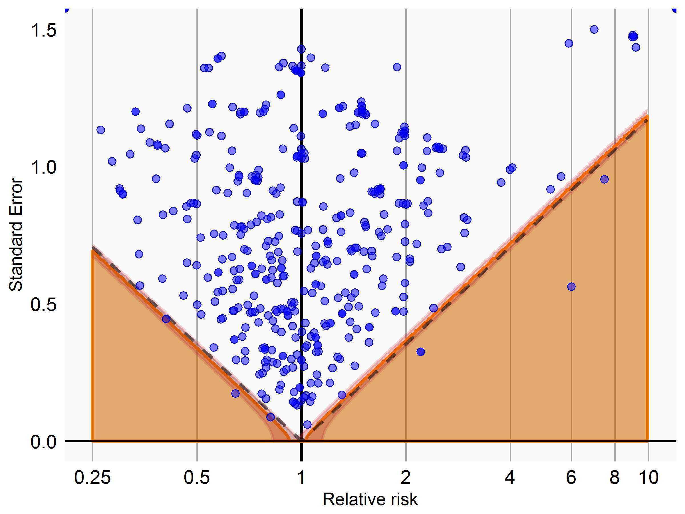
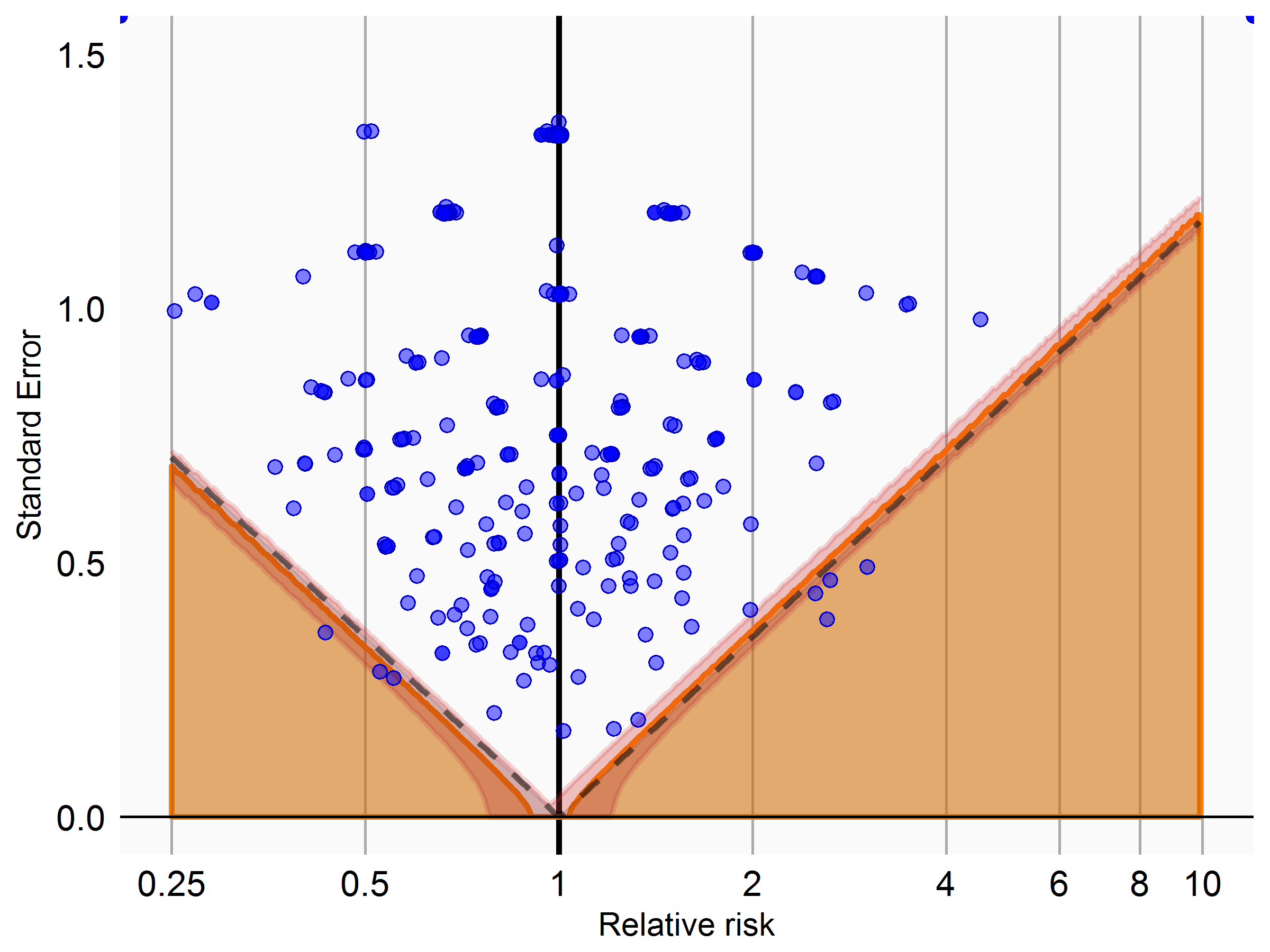
I used information from clinicaltrials.gov to identify completed randomized trials with a placebo control. For all potential adverse events reported in the studies, I then applied our current process for classifying drug-outcome pairs as negative controls. For those deemed negative controls, I then used the counts reported in clinicaltrials.gov to compute the effect size, and evaluated whether these effect sizes were consistent with the null being true. Below is the plot for non-serious effects (top) and serious (bottom) effects:
What these are showing is that the null appears to be exactly true for those that match our criteria for negative controls. I know there’s some circularity here (effects observed in a trial would be mentioned in the label, which is one source we use to classify things as negative controls), but at least it gives me some consolation.
I cannot find what exactly is Alejandro’s method on the forum. Is it to drop existing outcomes but still inject outcomes according to Martijn’s method. In the past, we had proposed doing Martijn’s method two ways, one where you add the new signals on top of the old ones, and one where you drop the old ones with purely injected signals. The plan was to compare the two to determine the algorithm’s sensitivity to that factor. We would hope to see little difference.
Or is Alejandro’s method to drop variables from the analysis to convert measured confounding to unmeasured confounding. Or is it some other method?
I would expect to see little difference in confounding structure between positive and negative controls because the effects are so small, UNLESS an effect is already suspected by doctors or proven.
What does the statement that a negative control is “exactly null” or “perfectly true” mean? That there is really no effect, that the effect estimate is 1.000, or that the CI covers 1?
In discussions at the end of the F2F, there was concern equating unmeasured confounding with measured confounding that was forced to be unmeasured (e.g., by forgetting variables), assuming the former was more complicated than the latter.
Alejandro has a nice whitepaper on his method that he shared with me, but since it’s not published I don’t know whether he can share it further. In a nutshell Alejandro’s approach is both things you mentioned:
Start with a blank slate, and generate all outcomes using a model fitted on the real data
Drop covariates from the data available to the method to simulate unmeasured confounding
Alejandro also has some nice extensions in his paper for example for simulating effect heterogeneity.
What I meant by the negative controls being ‘exactly null’ was that there is really no effect, and therefore the true relative risk is exactly 1. This is a necessary condition for our method evaluation and calibration to work.
Correct me if I’m wrong, but for the scenario where we want to evaluate method’s ability to answer the question:
What is the change in risk of outcome X due to exposure to A?
I guess the simulation won’t work. A specific example: if we want to evaluate the Self-Controlled Case Series design, there aren’t the two groups for which we can generate outcomes from scratch.
My algorithm is designed with a new-user cohort study in mind since it is probably the most widely-applicable and widely-used design. However, I think that mechanically it would be possible to force data from a self-controlled case series into an amenable format, it would just be a matter of saying what are the covariates for the patient and their “control”.
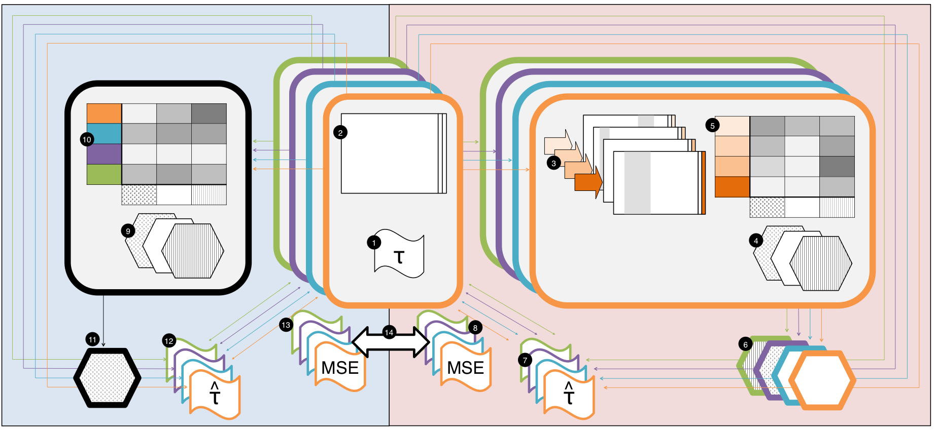
A gold-standard set of RCTs is assembled and corresponding treatment effects are recorded.
For each trial question, the EHR is used to create a corresponding observational dataset
Each observational dataset is used to create a slate of semi-simulated datasets with different treatment effects and hidden confounding
A battery of causal inference methods is applied to each semi-simulated dataset
Each method produces a treatment effect estimate which is compared to the true effect set by the user to generate the semi-simulated dataset
The causal inference method with the smallest errors across a variety of simulations is chosen for the final analysis of each trial question
The question-specific best method is used on the corresponding observational dataset to estimate a treatment effect for each RCT question
The effect estimates are compared to the RCT estimates to obtain a measure of error
The battery of causal inference methods is applied to each observational dataset
Each method produces a treatment effect estimate which is compared to the true effect as measured by the RCT
The causal inference method with the smallest errors across all RCT questions is chosen for the final analysis of each trial question
The overall best causal inference method is used on each observational dataset to estimate a treatment effect for each RCT question
The effect estimates are compared to the RCT estimates to obtain a measure of error
The errors from the two meta-evaluations are aggregated and compared to assess whether there is utility in discovering the causal inference methods that work best for each dataset or if we do just as well using a single one-size-fits-all method
Conceptually, we could imagine adding three other arms to this, which would be:
a question-specific injected-outcomes evaluation
a one-size-fits-all injected-outcomes evaluation
and a one-size-fits-all simulated-outcomes evaluation
Is our fitting just RCT-specific or also database-specific? That is, say one of the RCTs includes a variable that for two patients happens to mess up any attempt to do a self-controlled case series study. You go through the process on the right and it concludes SCCS don’t work, and you pick another method. But really SCCS was the right method. We just got unlucky on the database.
Put another way, can the question-specific approach produce overfitting? And does this evaluation measure that?
Maybe use some kind of leave one out cross validation on the datasets. Pick a method on N-1 and test on the Nth, comparing one-size to question-specific.
I think there currently is danger of overfitting, but I’m sure Alejandro just left out a train-test split to keep it simple(r).
I’m not sure we’ll have enough viable RCTs for this, but if we do it would be cool
One way I’m thinking about it is that you’re effectively proposing a meta-method: a method that is a combination of generating question-specific test data, finding the optimal method (from a battery of methods) on that data, and applying the optimal method to the question at hand. We can compare this meta-method against any individual other method, or specifically against a one-size-fits-all method (the method that works good on average on an out-of-sample gold standard).
@hripcsa: yes, we would do this in multiple databases and then the final comparison in step 14 would be a meta-analysis (you could imagine maybe having a random effect to capture the inter-database variability).
@schuemie: bingo! It is a meta-method, and this whole thing is a meta-evaluation.
And yes, the one-size-fits-all method would be determined on a training set of RCTs, and the errors would be evaluated on a test set of RCTs. For the question-specific meta-method the training data are the simulated datasets that come from the test set data, and the test set is the same.
Also, to do a one-size-fits-all evaluation with the simulated outcomes approach all that would be necessary is to concatenate all the tables (label 5) of the RCTs together (like 4 orange rows, 4 teal rows, 4 purple rows, etc). And a question-specific evaluation using real data would be done by subsetting the table (label 10) by some kind of “question type” or similarity (but as we discussed that’s probably too hard to figure out). All that just to say that the figure really does capture a lot!
@schuemie how many RCTs do you think would be necessary to make it viable? I don’t mean literally a number, I just want to explore your thoughts here. This is more or less my plan moving forward.
We’ve settled (for now) on using signal injection (on top of negative controls) for synthesizing positive controls. The next question becomes: what should be the shape of the effect?
For those of you who remember OSIM2, there we implemented the following types of signal:
Acute: the hazard is increased with a constant factor (over baseline) for the first 30 days following exposure start
Insidious: the hazard is increased with a constant factor (over baseline) while exposed
Cumulative: the hazard is increased with a factor that grows with cumulative exposure (measured in days). This factor is maintained (but does not grow further) when someone stops being exposed.
What I currently have implemented is the equivalent of Insidious.
To some extent the choice is arbitrary, since we probably only want to evaluate methods that use a risk window that is consistent with the injected signal shape. But some methods might be better equipped to detect certain types of effects, such as our Exposure-adjusted SCCS which was specifically designed to detect cumulative effects.
On signal profile, I would assume “insidious,” but I would rename it. The definition of insidious is hidden (and gradual) but still cumulative: the chance for harm grows over time. Maybe just call it “constant,” but you also have to convey that it stops when the drug stops. Another name would be “proportional,” which means proportional to dose, with risk dropping to zero when the dose does. But we are not measuring dose.