Team:
For those who missed any of the fun in Phenotype Phebruary Week 1, here’s a page with a running inventory of the phenotype conversations we’ve started: Phenotype Phebruary Daily Updates – OHDSI As we embark on Week 2 of Phenotype Phebruary, I decided to select a phenotype that was highly voted on by our community that was more surprising to me. I don’t know why kidney stones were of such interest to so many of you, but the community has spoken and I like the challenge of coming up with a fun and compelling story to promote phenotyping, so here goes…
Clinical description:
Kidney stone disease occurs when a calculus develops in the urinary tract, often starting in the kidney and passing through the ureters, bladder and urethra. This phenomenon, also known as neprolithiasis or urolithiasis, can be asymptomatic if the kidney stones are small enough. However, the size, shape and composition of calculi can vary substantially, and larger stones can create obstructions at any stage across the urinary tract. Such blockages can cause acute pain, typically presenting in the lower back or abdomen, and may also cause painful urination or hematuria. Kidney stones are typically diagnosed by symptoms, urine tests and imaging. Treatment often is based on patient symptoms. Pain management and hydration can allow some stones to pass spontaneously. Drugs to expedite passage, such as alpha blockers and calcium channel blockers, can be considered. Shock wave lithotripsy can be used in some circumstances to break stone into smaller pieces. Surgical removal via nephrolithotomy or ureteroscopy may be indicated depending on stone size and patient comorbidities and pain intensity.
Phenotype development:
One of the surprising statistics that I read across many different references was the notion that half of the people who have had a kidney stone will have another 10 years. This number was thrown around in many publications, and yet most cited the same seminal paper: Uribarri et al, “The first kidney stone”, from BMJ in 1989. That paper provides a review of past studies that examined recurrence of kidney stones, providing their Table 1 compilation of the identified studies:

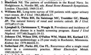
There were six papers cited as sources for this meta-analysis. Here are the specific citations:

Now, I don’t know about you, but I’m not fully comfortable generalizing for the experience of sailors in the Royal Navy prior to 1969 to my cushy sedentary lifestyle here in 2022. But, the pattern shown across these studies show some notion of an expectation that ~10-20% of patients with a kidney stone can expect a recurrence in 1 year, 25-50% will have a recurrence in 5 years, and 37-67% may have a recurrence in 10 years.
So, with this data point in context, I was surprised to read Alexander et al, “Kidney stones and kidney function loss: a cohort study” in BMJ in 2012. In their paper, they described their phenotype for kidney stones, to be applied their Alberta Kidney Disease Network database:
“We used physician claims, data on use of hospitalisation and ambulatory care, and ICD-9 codes (592, 594, 274.11) and ICD-10 codes (N20.0, N20.1, N20.2, N20.9, N21.0, N21.1, N21.8, N21.9, N22.0, N22.8) to identify presentations of kidney stones. The accuracy of these codes in defining a kidney stone episode has been validated.12 One or more of these codes in any position for any inpatient or outpatient claim was taken to represent an episode of kidney stones. We assumed that an interval of a year or more between claims represented separate kidney stone episodes; claims occurring within a year of each other were classified as a result of a single stone episode.16 17”.
What I particularly took note of is “we assumed an interval of a year or more between claims represented separate kidney stone episodes”, because Uribarri’s results suggest that this assumption would stimulate substantial event misclassification, with recurrent events being bundled with the original event.
Which brings us to the phenotype development methodological question: how do we model recurrent events, balancing the potential errors of falsely combining together separate events into a single episode vs. the risk of falsely counting events as independent episodes when they are in fact markers of continuation of care for the same health experience?
To answer that question: Let’s create some phenotypes and empirically evaluate the consequences!
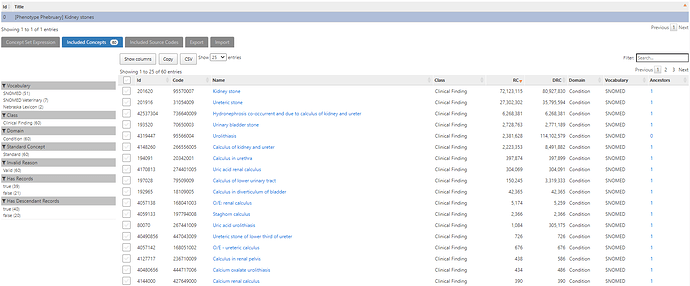
First, the conceptset for kidney stones. Turns out that its pretty straightforward, using literature as a starting reference, using the vocabulary hierarchies and PHOEBE recommendations:
This simple conceptset resolves to 60 concepts, but <10 are driving the cohort based on record count. the main one being ‘Kidney stone’:
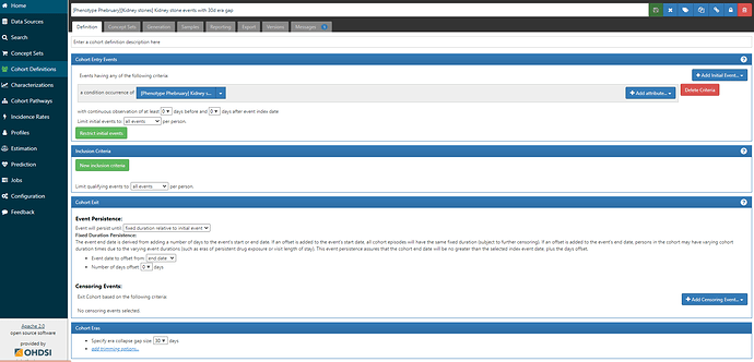
The logic for the cohort is also straightforward, we take all events of a condition occurence of the ‘Kidney stone’ conceptset:
But, I’ll draw your attention to the last line of that screenshot: Cohort Eras → Specify era collapse gap size = 30 days. This means that if successive observed are within 30 days of one another, they will be collapsed together into a single episode. There must be a gap of >30 days in order for two events to be identified as separate episodes.
But, how do we decide on the era collapse gap size? This is whether clinical knowledge and understanding of the biological phenomenon is useful, but also one needs to understand how healthcare data may be captured for the clinical event of interest. Small stones may pass spontaneously in 4 weeks, so 30 days would cover this duration, but may not necessarily cover the duration from first presenting symptom and complete resolution. But, Alexander et al’s assumption that the gap size should be 365d means that recurrences within 1 year are not possible (in spite of evidence supporting the contrary).
What can we do? Test the impact of multiple alternative gap size windows on the number of events that are identified. The number of persons with at least one event will remain the same, but the number of events per person can shift substantially.
For this exercise, I created three phenotypes for kidney stones, the links to ATLAS-phenotype are below:
- [Phenotype Phebruary][Kidney stones] Kidney stone events with 30d era gap
- [Phenotype Phebruary][Kidney stones] Kidney stone events with 90d era gap
- [Phenotype Phebruary][Kidney stones] Kidney stone events with 365d era gap
I evaluated these 3 phenotypes against the IBM MarketScan CCAE database.
First, I calculated how many events each person in the cohort had, across each definition, and then summarized the number of persons by number of events. I did this via direct SQL on the COHORT table that is populated by ATLAS in the RESULTS schema:
create table #kidney_stone_events as
select *, case when cohort_definition_id = 5291 then 'Kidney stone with 30d era'
              when cohort_definition_id = 5292 then 'Kidney stone with 90d era'
              when cohort_definition_id = 5293 then 'Kidney stone with 365d era'
              else 'Other' end as cohort_name
from cohort
where cohort_definition_id in (5291, 5292, 5293)
;

--find number of persons, by number of unique events, within each cohort definition
select num_events,
    max(case when cohort_name = 'Kidney stone with 30d era' then num_persons else 0 end) as num_persons_30d,
    max(case when cohort_name = 'Kidney stone with 90d era' then num_persons else 0 end) as num_persons_90d,
    max(case when cohort_name = 'Kidney stone with 365d era' then num_persons else 0 end) as num_persons_365d
from
(
select cohort_name, num_events, count(subject_id) as num_persons
from
(
select cohort_name, subject_id, min(cohort_start_date) as first_event_date, count(subject_id) as num_events
from #kidney_stone_events
group by cohort_name, subject_id
) t1
group by cohort_name, num_events
) t2
group by num_events
;
And the results show that the era gap window does have a substantial impact on the number of events observed per person, take a look at the tail of this distribution:
| num_events | num_persons_30d | num_persons_90d | num_persons_365d |
|---|---|---|---|
| 1 | 2036018 | 2271273 | 2668675 |
| 2 | 558099 | 512921 | 392894 |
| 3 | 245649 | 196161 | 97258 |
| 4 | 129054 | 92984 | 30028 |
| 5 | 75295 | 49807 | 10426 |
| 6 | 47471 | 28971 | 3778 |
| 7 | 31048 | 17520 | 1284 |
| 8 | 21430 | 11319 | 456 |
| 9 | 14840 | 7574 | 155 |
| 10 | 10792 | 4906 | 67 |
| 11 | 8149 | 3451 | 20 |
| 12 | 5801 | 2373 | 8 |
| 13 | 4532 | 1648 | 1 |
| 14 | 3495 | 1174 | 0 |
| 15 | 2762 | 861 | 0 |
| 16 | 2070 | 585 | 0 |
| 17 | 1653 | 418 | 0 |
| 18 | 1344 | 316 | 0 |
| 19 | 1090 | 228 | 0 |
| 20 | 811 | 175 | 0 |
| 21 | 620 | 119 | 0 |
| 22 | 524 | 89 | 0 |
| 23 | 422 | 49 | 0 |
| 24 | 350 | 47 | 0 |
| 25 | 285 | 23 | 0 |
| 26 | 245 | 18 | 0 |
| 27 | 201 | 14 | 0 |
| 28 | 165 | 8 | 0 |
| 29 | 126 | 7 | 0 |
| 30 | 121 | 3 | 0 |
| 31 | 107 | 6 | 0 |
| 32 | 66 | 1 | 0 |
| 33 | 63 | 1 | 0 |
| 34 | 52 | 0 | 0 |
| 35 | 47 | 0 | 0 |
| 36 | 43 | 0 | 0 |
| 37 | 36 | 0 | 0 |
| 38 | 27 | 0 | 0 |
| 39 | 23 | 0 | 0 |
| 40 | 14 | 0 | 0 |
| 41 | 9 | 0 | 0 |
| 42 | 11 | 0 | 0 |
| 43 | 12 | 0 | 0 |
| 44 | 13 | 0 | 0 |
| 45 | 11 | 0 | 0 |
| 46 | 10 | 0 | 0 |
| 47 | 9 | 0 | 0 |
| 48 | 7 | 0 | 0 |
| 49 | 5 | 0 | 0 |
| 50 | 3 | 0 | 0 |
| 51 | 3 | 0 | 0 |
| 52 | 4 | 0 | 0 |
| 53 | 4 | 0 | 0 |
| 54 | 1 | 0 | 0 |
| 55 | 1 | 0 | 0 |
| 56 | 4 | 0 | 0 |
| 59 | 1 | 0 | 0 |
| 62 | 1 | 0 | 0 |
| 70 | 1 | 0 | 0 |
Given this, we can expect that the recurrence rate would vary by the gap window length. But how much? Here’s a simple query to estimate the recurrence rate at 1 year, 5 year, and 10 year intervals (similar to the original Uribarri paper). Note, we require persons to be observed for the full time-at-risk to be included, which is why the denominators shift lower as the interval is enlargened:
--estimate recurrence proportions at 1/5/10 year intervals
select '1. 1 year recurrence proportion' as time_at_risk,
    first_events.cohort_name,
    count(distinct first_events.subject_id) as num_persons_at_risk,
    count(distinct kse1.subject_id) as num_persons_w_event,
    1.0*count(distinct kse1.subject_id) / count(distinct first_events.subject_id) as pct_persons_w_event
from
(
select cohort_name, subject_id, min(cohort_start_date) as first_event_date
from #kidney_stone_events
group by cohort_name, subject_id
) first_events
inner join observation_period op1
on first_events.subject_id = op1.person_id
and first_events.first_event_date >= dateadd(day,365,op1.observation_period_start_date)
and first_events.first_event_date <= dateadd(day,-365,op1.observation_period_end_date)
left join #kidney_stone_events kse1
on first_events.cohort_name = kse1.cohort_name
and first_events.subject_id = kse1.subject_id
and first_events.first_event_date < kse1.cohort_start_date
and dateadd(day,365,first_events.first_event_date) >= kse1.cohort_start_date
group by first_events.cohort_name

union all

select '2. 5 year recurrence proportion' as time_at_risk,
    first_events.cohort_name,
    count(distinct first_events.subject_id) as num_persons_at_risk,
    count(distinct kse1.subject_id) as num_persons_w_event,
    1.0*count(distinct kse1.subject_id) / count(distinct first_events.subject_id) as pct_persons_w_event
from
(
select cohort_name, subject_id, min(cohort_start_date) as first_event_date
from #kidney_stone_events
group by cohort_name, subject_id
) first_events
inner join observation_period op1
on first_events.subject_id = op1.person_id
and first_events.first_event_date >= dateadd(day,365,op1.observation_period_start_date)
and first_events.first_event_date <= dateadd(day,-365*5,op1.observation_period_end_date)
left join #kidney_stone_events kse1
on first_events.cohort_name = kse1.cohort_name
and first_events.subject_id = kse1.subject_id
and first_events.first_event_date < kse1.cohort_start_date
and dateadd(day,365*5,first_events.first_event_date) >= kse1.cohort_start_date
group by first_events.cohort_name


union all

select '3. 10 year recurrence proportion' as time_at_risk,
    first_events.cohort_name,
    count(distinct first_events.subject_id) as num_persons_at_risk,
    count(distinct kse1.subject_id) as num_persons_w_event,
    1.0*count(distinct kse1.subject_id) / count(distinct first_events.subject_id) as pct_persons_w_event
from
(
select cohort_name, subject_id, min(cohort_start_date) as first_event_date
from #kidney_stone_events
group by cohort_name, subject_id
) first_events
inner join observation_period op1
on first_events.subject_id = op1.person_id
and first_events.first_event_date >= dateadd(day,365,op1.observation_period_start_date)
and first_events.first_event_date <= dateadd(day,-365*10,op1.observation_period_end_date)
left join #kidney_stone_events kse1
on first_events.cohort_name = kse1.cohort_name
and first_events.subject_id = kse1.subject_id
and first_events.first_event_date < kse1.cohort_start_date
and dateadd(day,365*10,first_events.first_event_date) >= kse1.cohort_start_date
group by first_events.cohort_name

;
In CCAE, this provide us kidney stone recurrence proportions as follows:
| time_at_risk | cohort_name | num_persons_at_risk | num_persons_w_event | pct_persons_w_event |
|---|---|---|---|---|
| 1. 1 year recurrence proportion | Kidney stone with 30d era | 1276749 | 341312 | 0.27 |
| 1. 1 year recurrence proportion | Kidney stone with 90d era | 1276749 | 213682 | 0.17 |
| 1. 1 year recurrence proportion | Kidney stone with 365d era | 1276749 | 0 | 0.00 |
| 2. 5 year recurrence proportion | Kidney stone with 30d era | 352293 | 163280 | 0.46 |
| 2. 5 year recurrence proportion | Kidney stone with 90d era | 352293 | 144931 | 0.41 |
| 2. 5 year recurrence proportion | Kidney stone with 365d era | 352293 | 110024 | 0.31 |
| 3. 10 year recurrence proportion | Kidney stone with 30d era | 80623 | 45454 | 0.56 |
| 3. 10 year recurrence proportion | Kidney stone with 90d era | 80623 | 42458 | 0.53 |
| 3. 10 year recurrence proportion | Kidney stone with 365d era | 80623 | 37921 | 0.47 |
So, we can see that the gap size window has a substantial impact on 1 year recurrence; by definition, a 365d gap window means that no recurrence is possible, but the recurrence proportion varies from 17% for a 90d gap window to 27% for a 30d gap window. The 5-year recurrence proportions range from 31% for 365d gap to 46% for the 30d gap. And the 10-year recurrence proportion ranges from 47% for 365d gap to 56% for 30d gap. So the impact of gap window decreases as you expand the time-at-risk window.
Remarkably, the real-world experience in the privately insured population of the CCAE claims dataset through 2021 is not altogether different from those of sailors in the Royal Navy pre-1969 or Minnesotans pre-1979.
My takeaways from this exercise: defining kidney stone events reinforces the need to follow the OHDSI definition of a cohort: a set of persons satisfying one or more criteria for a duration of time. While it is critically important to define the entry events and inclusion criteria correctly, it is equally important to pay attention to the cohort exit strategy, and ensure that you are appropriately modeling when episodes are expected to be over. In this case, kidney stone entry events were straightforward to implement, but the exit strategy used to collapse episodes had a major impact on estimates of recurrence.
How do you think about modeling recurrent events when phenotyping? What do you consider when weighing the tradeoff of ‘false positive’ events where a case is really a follow-up from a prior episode vs. the ‘false negative’ of collapsing together events that are truly independent events? What empirical diagnostics should we put in place to evaluate this tradeoff?


