Hi @Nathaniel_Phillips,
I’ll try to explain as best I can but I don’t fully understand the logic behind the inclusion rule mask yet. It just hasn’t “clicked” for me yet. But here we go…
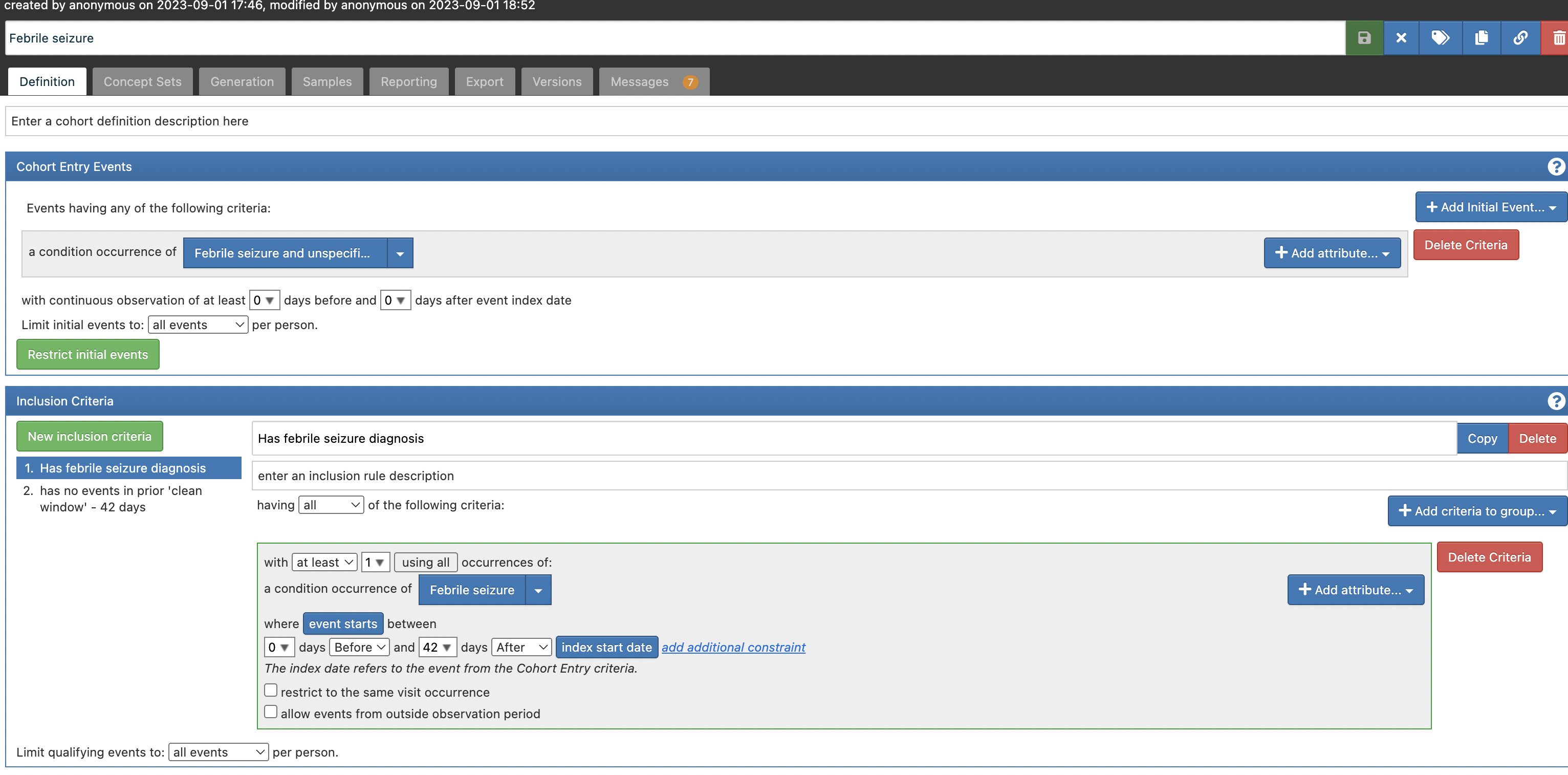
Let’s use a cohort from the phenotype library “Febrile seizure”.
https://atlas-demo.ohdsi.org/#/cohortdefinition/1785335/definition
This cohort has two inclusion rules.
I generated this cohort on a test database I use with the following code.
library(DatabaseConnector)
library(dplyr)
connectionDetails <- createConnectionDetails(
dbms = "sql server",
server = Sys.getenv("CDM5_SQL_SERVER_SERVER"),
user = Sys.getenv("CDM5_SQL_SERVER_USER"),
password = Sys.getenv("CDM5_SQL_SERVER_PASSWORD"),
port = Sys.getenv("CDM5_SQL_SERVER_PORT")
)
connection <- connect(connectionDetails)
cohortDatabaseSchema <- Sys.getenv("CDM5_SQL_SERVER_SCRATCH_SCHEMA")
cdmDatabaseSchema <- Sys.getenv("CDM5_SQL_SERVER_CDM_SCHEMA")
# just generate one cohort
cohortDefinitionSet <- PhenotypeLibrary::listPhenotypes() %>%
dplyr::pull("cohortId") %>%
PhenotypeLibrary::getPlCohortDefinitionSet() %>%
dplyr::filter(cohortId == 54)
readr::write_file(cohortDefinitionSet$json, here::here("Febrile seizure.json"))
cohortTableNames <- CohortGenerator::getCohortTableNames(cohortTable = "pl_cohort")
# Next create the tables on the database
CohortGenerator::createCohortTables(
connectionDetails = connectionDetails,
cohortTableNames = cohortTableNames,
cohortDatabaseSchema = cohortDatabaseSchema,
incremental = FALSE
)
# Generate the cohort set
CohortGenerator::generateCohortSet(
connectionDetails = connectionDetails,
cdmDatabaseSchema = cdmDatabaseSchema,
cohortDatabaseSchema = cohortDatabaseSchema,
cohortTableNames = cohortTableNames,
cohortDefinitionSet = cohortDefinitionSet,
incremental = FALSE
)
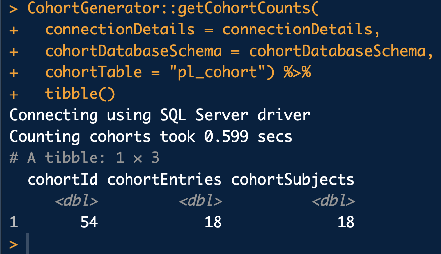
CohortGenerator::getCohortCounts(
connectionDetails = connectionDetails,
cohortDatabaseSchema = cohortDatabaseSchema,
cohortTable = "pl_cohort") %>%
tibble()
We can see the cohort ends up with 18 entries (rows) and 18 subjects (people). Remeber that a person can have multiple entries in the same cohort since they can enter, exit, and then reenter at a later time.
Next I will download the cohort inclustion result table from the database.
con <- connect(connectionDetails)
# Bring the inclusion result table to R memory
inclusionResult <- querySql(con, glue::glue("select * from {cohortDatabaseSchema}.pl_cohort_inclusion_result")) %>%
dplyr::rename_all(tolower) %>%
dplyr::mutate(inclusion_rule_mask = as.numeric(.data$inclusion_rule_mask)) %>%
tibble()
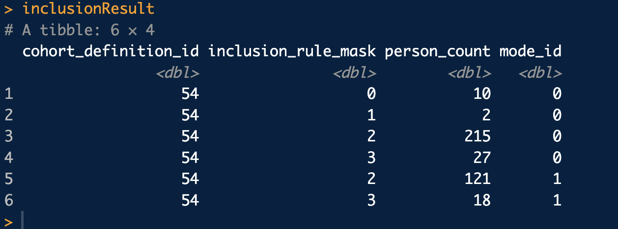
inclusionResult
So this table is a bit cryptic to understand but contains the information you need to build an attrition table. By summing various combination of rows in this table you can get at all the various combinations of inclusion rules. It will allow you to calculate the number of subjects and records for any combination of inclusion rules.
Now my colleague Marti wrote a nice helper function to give you the inclusion rule mask ids for each inclusion rule. And actually Marti deserves the credit for all of this investigative work and spent a lot of time trying to understand these cohort tables. The function is
getInclusionMaskId <- function(numberInclusion) {

  inclusionMaskMatrix <- dplyr::tibble(
    inclusion_rule_mask = 0:(2^numberInclusion - 1)
  )

  for (k in 0:(numberInclusion - 1)) {
    inclusionMaskMatrix <- inclusionMaskMatrix %>%
      dplyr::mutate(!!paste0("inclusion_", k) :=
                      rep(c(rep(0, 2^k), rep(1, 2^k)), 2^(numberInclusion - k - 1))
      )
  }

  lapply(-1:(numberInclusion - 1), function(x) {
    if (x == -1) {
      return(inclusionMaskMatrix$inclusion_rule_mask)
    } else {
      inclusionMaskMatrix <- inclusionMaskMatrix
      for (k in 0:x) {
        inclusionMaskMatrix <- inclusionMaskMatrix %>%
          dplyr::filter(.data[[paste0("inclusion_", k)]] == 1)
      }
      return(inclusionMaskMatrix$inclusion_rule_mask)
    }
  })
}
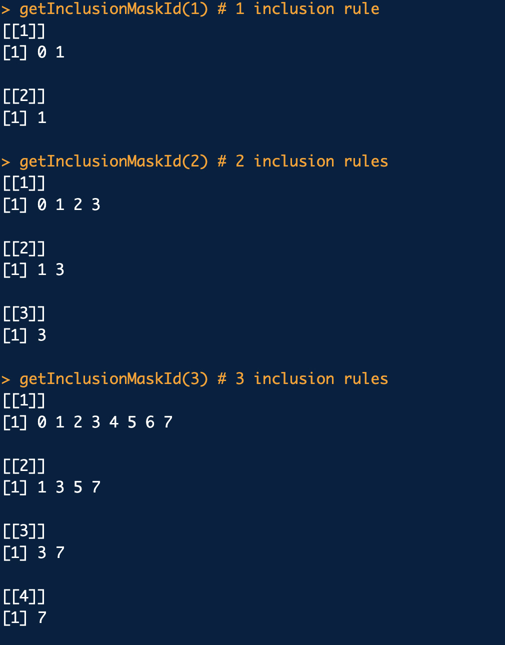
You pass in the number of inclusion rules you have and it will return a list of the same length with the mask ids you need to use.
Here is some example output.
Next I’ll extract the names of the inclusion rules from the cohort definition.
# get the text descriptions of the inclusion rules
cohortDefinition <- jsonlite::fromJSON(cohortDefinitionSet$json[1], simplifyVector = FALSE)
str(cohortDefinition, max.level = 1)
inclusionNames <- purrr::map_chr(cohortDefinition$InclusionRules, "name")
inclusionNames
Create a list of dataframes using the appropriate inclusion rule mask ids
numberInclusionRules <- length(inclusionNames)
inclusionMaskId <- getInclusionMaskId(numberInclusionRules)
inclusionNames <- c("Qualifying initial records", inclusionNames)
attrition <- list()

id <- 54 # cohort definition id

for (k in 1:(numberInclusionRules + 1)) {

  number_records <- inclusionResult %>%
    dplyr::filter(.data$cohort_definition_id == id) %>%
    dplyr::filter(.data$mode_id == 0) %>%
    dplyr::filter(.data$inclusion_rule_mask %in% inclusionMaskId[[k]]) %>%
    dplyr::pull("person_count") %>%
    base::sum()

  number_subjects = inclusionResult %>%
    dplyr::filter(.data$cohort_definition_id == id) %>%
    dplyr::filter(.data$mode_id == 1) %>%
    dplyr::filter(.data$inclusion_rule_mask %in% inclusionMaskId[[k]]) %>%
    dplyr::pull("person_count") %>%
    base::sum()

  attrition[[k]] <- dplyr::tibble(
    cohort_definition_id = id,
    number_records = number_records,
    number_subjects = number_subjects,
    reason_id = k,
    reason = inclusionName[k]
  )
}
Finally bind these together and compute the number dropped at each step.
attrition <- attrition %>%
dplyr::bind_rows() %>%
dplyr::mutate(
excluded_records =
dplyr::lag(.data$number_records, 1, order_by = .data$reason_id) -
.data$number_records,
excluded_subjects =
dplyr::lag(.data$number_subjects, 1, order_by = .data$reason_id) -
.data$number_subjects
) %>%
dplyr::mutate(
excluded_records = dplyr::coalesce(.data$excluded_records, 0),
excluded_subjects = dplyr::coalesce(.data$excluded_subjects, 0)
)
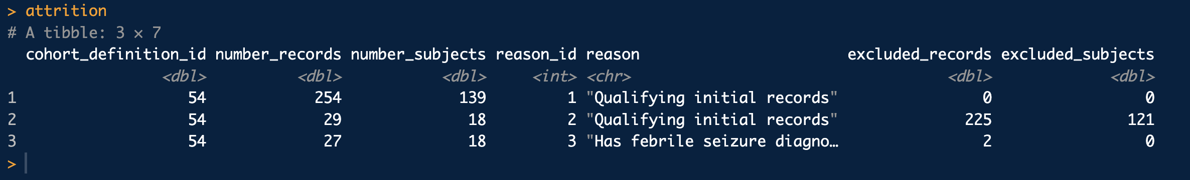
attrition
And voila! that’s all you need to do! There might be an easier way to do this but I’m not sure. And I’m sure I botched this explanation pretty good. Maybe @Chris_Knoll or @anthonysena can fill in the gaps or correct anything I got wrong.
Great question!